{HCNA-AI 数学知识}之其他实验

​4.1最小二乘法实现

4.1.1算法介绍

最小二乘法（Least Square Method），做为分类回归算法的基础，有着悠久的历史。它通过最小化误差的平方和寻找数据的最佳函数匹配。利用最小二乘法可以简便地求得未知的参数，并使得预测的数据与实际数据之间误差的平方和为最小。

4.1.2代码实现

# 代码输入：

import numpy as np # 引 入 numpy

import scipy as sp import pylab as pl

from scipy.optimize import leastsq # 引入最小二乘函数

n = 9 # 多项式次数

# 目标函数

def real_func(x):

return np.sin(2 * np.pi * x)

# 多项式函数

def fit_func(p, x):

f = np.poly1d(p) return f(x)

# 残差函数

def residuals_func(p, y, x): ret = fit_func(p, x) - y return ret

x = np.linspace(0, 1, 9) # 随机选择 9 个点作为 x

x_points = np.linspace(0, 1, 1000) # 画图时需要的连续点

y0 = real_func(x) # 目标函数

y1 = [np.random.normal(0, 0.1) + y for y in y0] # 添加正太分布噪声后的函数

p_init = np.random.randn(n) # 随机初始化多项式参数

plsq = leastsq(residuals_func, p_init, args=(y1, x))

print('Fitting Parameters: ', plsq[0]) # 输出拟合参数

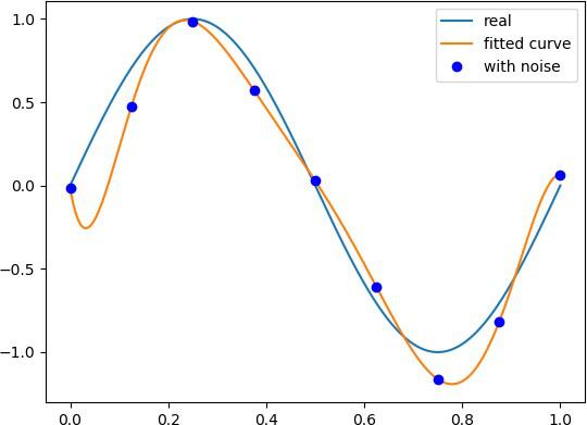
pl.plot(x_points, real_func(x_points), label='real') pl.plot(x_points, fit_func(plsq[0], x_points), label='fitted curve') pl.plot(x, y1, 'bo', label='with noise')

pl.legend() pl.show()

# 结果输出：

Fitting Parameters: [-1.22007936e+03 5.79215138e+03 -1.10709926e+04 1.08840736e+04

-5.81549888e+03 1.65346694e+03 -2.42724147e+02 1.96199338e+01

-2.14013567e-02]

# 可视化图像：

4.2 梯度下降法实现

4.2.1 算法介绍

梯度下降法（gradient descent），又名最速下降法，是求解无约束最优化问题最常用的方法，它是一种迭代方法，每一步主要的操作是求解目标函数的梯度向量，将当前位置的负梯度方向作为搜索方向（因为在该方向上目标函数下降最快，这也是最速下降法名称的由来）。

梯度下降法特点：越接近目标值，步长越小，下降速度越慢。

4.2.2 代码实现

# 代码输入：

# 训练集

# 每个样本点有 3 个分量 (x0,x1,x2)

x = [(1, 0., 3), (1, 1., 3), (1, 2., 3), (1, 3., 2), (1, 4., 4)]

# y[i] 样本点对应的输出

y = [95.364, 97.217205, 75.195834, 60.105519, 49.342380]

# 迭代阀值，当两次迭代损失函数之差小于该阀值时停止迭代

epsilon = 0.0001

# 学习率

alpha = 0.01

diff = [0, 0]

max_itor = 1000

error1 = 0

error0 = 0

cnt = 0

m = len(x)

# 初始化参数

theta0 = 0

theta1 = 0

theta2 = 0

while True:

cnt += 1

# 参数迭代计算

for i in range(m):

# 拟合函数为 y = theta0 * x[0] + theta1 * x[1] +theta2 * x[2]

# 计算残差

diff[0] = (theta0 + theta1 * x[i][1] + theta2 * x[i][2]) - y[i]

# 梯 度 = diff[0] * x[i][j]

theta0 -= alpha * diff[0] * x[i][0] theta1 -= alpha * diff[0] * x[i][1] theta2 -= alpha * diff[0] * x[i][2]

# 计算损失函数

error1 = 0

for lp in range(len(x)):

error1 += (y[lp]-(theta0 + theta1 * x[lp][1] + theta2 * x[lp][2]))**2/2

if abs(error1-error0) < epsilon: break

else:

error0 = error1

print(' theta0 : %f, theta1 : %f, theta2 : %f, error1 : %f' % (theta0, theta1, theta2, error1) )

print('Done: theta0 : %f, theta1 : %f, theta2 : %f' % (theta0, theta1, theta2) )

print('迭代次数: %d' % cnt )

# 结果输出：

theta0 : 2.782632, theta1 : 3.207850, theta2 : 7.998823, error1 : 5997.941160

theta0 : 4.254302, theta1 : 3.809652, theta2 : 11.972218, error1 : 3688.116951

theta0 : 5.154766, theta1 : 3.351648, theta2 : 14.188535, error1 : 2889.123934

theta0 : 5.800348, theta1 : 2.489862, theta2 : 15.617995, error1 : 2490.307286

theta0 : 6.326710, theta1 : 1.500854, theta2 : 16.676947, error1 : 2228.380594

theta0 : 6.792409, theta1 : 0.499552, theta2 : 17.545335, error1 : 2028.776801

… …

theta0 : 97.717864, theta1 : -13.224347, theta2 : 1.342491, error1 : 58.732358

theta0 : 97.718558, theta1 : -13.224339, theta2 : 1.342271, error1 : 58.732258

theta0 : 97.719251, theta1 : -13.224330, theta2 : 1.342051, error1 : 58.732157

Done: theta0 : 97.719942, theta1 : -13.224322, theta2 : 1.341832

迭代次数: 2608